The goal of this project is to gain insight into the dynamic behavior of the immune system. Check stability of fixed points via Lyapunov stability analysis. Simulations with the use of MATLAB have been performed for the original system as well as the time-delayed system. Three clinical conditions are given and the response of the immune system is determined for each of them. For condition 3 also a time-delayed system is simulated for which a Hopf bifurcation is determined. All feasible fixed points in all clinical conditions where asymptotically stable.
Introduction
Understanding the interaction between malignant cells and the immune system of an organism deserves quite some attention. A system theoretic perspective on this understanding proves quite useful for studying the dynamic features of tumor growth and to understand the implication on specific treatments. In fact, such a perspective brings valuable insight in some key mechanisms that are used in immunology, oncology and cancer biology. This will be the purpose of this project. The system of nonlinear coupled differential equations are given by:
\[\begin{aligned} &\dot{M}=1+a_1 M(1-M)-a_2 M H \\ &\dot{H}=a_3 H R-a_4 H \\ &\dot{R}=a_5 R(1-R)-a_6 H R-a_7 R \end{aligned}\]Where
- $M$ is the density of the malignant or tumor cells,
- $H$ is the density of the active hunting cells,
- $R$ is the density of the resting cells in the immune system.
All indicated parameters $a_i$ are non-negative numbers. In particular,
- $a_1$ is the growth rate of tumor cells,
- $a_2$ is the rate of destruction of tumor cells by the hunting cells,
- $a_3$ is the conversion rate from resting cells to hunting cells,
- $a_4$ is the natural death rate of hunting cells,
- $a_5$ is the growth rate of resting cells,
- $a_6$ is the conversion rate from hunting to resting cells,
- $a_7$ is the natural natural death rate of resting cells.
Fixed points and biological feasibility
The fixed points can be determined by solving the system of equations when the derivatives are zero, because the fixed points in a system are the solutions when there is no time dependency. Firstly, the rate of change of density of the hunting cells $\dot{H}=0$ is solved.
\[\begin{aligned} & a_3 H R-a_4 H=0 \\ & H(a_3 R-a_4)=0 \\ & H^{\ast}_1=0 \vee R^{\ast}_1=\frac{a_4}{a_3} \end{aligned}\]Where \(H^{\ast}_1\) will be substituted such that \(M^{\ast}_{1,\ 2}\) can be computed by solving $\dot{M}=0$.
\[\begin{aligned} & 1+a_1M(1-M)-a_2 M H=0 \\ & H^{\ast}_1=0\\ & 1+a_1 M-a_1 M^2=0 \\ & M^2-M -\frac{1}{a_1}\\ & M^{\ast}_{1,2}=\frac{1}{2}\pm\sqrt{\frac{1}{4}+\frac{1}{a_1}} \end{aligned}\]Next, $H^{\ast}_1$ is substituted while $\dot{R}=0$ to obtain $R_2$ and $R_3$:
\[\begin{aligned} & H^{\ast}_1=0\\ & a_5 R(1-R) - a_7 R=0 \\ & R(a_5-a_5 R -a_7)=0 \\ & R^{\ast}_2=0 \vee R^{\ast}_3=1-\frac{a_7}{a_5} \end{aligned}\]$H^{\ast}_2$ can be computed by implementing $R^{\ast}_1$ in $\dot{R}=0$:
\[\begin{aligned} & R^{\ast}_1=\frac{a_4}{a_3}\\ & a_5 R(1-R)-a_6 H R-a_7 R=0 \\ & \frac{a_4}{a_3}\cdot(a_5-a_5\cdot \frac{a_4}{a_3}-a_6\cdot H -a_7)=0 \\ & H^{\ast}_2=\frac{a_5 a_3 -a_4 a_5 -a_3 a_7}{a_3 a_6} \end{aligned}\]Finally, \(H^{\ast}_2\) can be substituted in the equation $\dot{M}=0$ to obtain $M_{3,4}$:
\[\begin{aligned} & H^{\ast}_2=\frac{a_5 a_3 -a_4 a_5 -a_3 a_7}{a_3 a_6}\\ & 1+a_1 M(1-M)-a_2 M H_2=0 \\ & M^{\ast}_{3,4}=(\frac{1}{2}-\frac{a_2}{2a_1}H_2^{\ast})\pm \sqrt{(\frac{a_2}{a_1}H_2-1)^2+\frac{1}{a_1}} \end{aligned}\]The resulting fixed points are stated below:
\[\begin{aligned} & (M^{\ast}_1,H^{\ast}_1,R^{\ast}_2)=(\frac{1}{2}+\sqrt{\frac{1}{4}+\frac{1}{a_1}},0,0)\\ & (M^{\ast}_2,H^{\ast}_1,R^{\ast}_2)=(\frac{1}{2}-\sqrt{\frac{1}{4}+\frac{1}{a_1}},0,0)\\ & (M^{\ast}_1,H^{\ast}_1,R^{\ast}_3)=(\frac{1}{2}+\sqrt{\frac{1}{4}+\frac{1}{a_1}},0,1-\frac{a_7}{a_5})\\ & (M^{\ast}_2,H^{\ast}_1,R^{\ast}_3)=(\frac{1}{2}-\sqrt{\frac{1}{4}+\frac{1}{a_1}},0,1-\frac{a_7}{a_5})\\ & (M^{\ast}_3,H^{\ast}_2,R^{\ast}_1)=\frac{1}{2}(\frac{a_2}{a_1}H_2^{\ast}-1)+ \sqrt{\frac{1}{4}\cdot(\frac{a_2}{a_1}H_2^{\ast}-1)^2+\frac{1}{a_1}},\frac{a_5 a_3 -a_4 a_5 -a_3 a_7}{a_3 a_6},\frac{a_4}{a_3})\\ & (M^{\ast}_4,H^{\ast}_2,R^{\ast}_1)=\frac{1}{2}(\frac{a_2}{a_1}H_2^{\ast}-1)- \sqrt{\frac{1}{4}\cdot(\frac{a_2}{a_1}H_2^{\ast}-1)^2+\frac{1}{a_1}},\frac{a_5 a_3 -a_4 a_5 -a_3 a_7}{a_3 a_6},\frac{a_4}{a_3})\\ \end{aligned}\]Feasibility
The positive invariant set \(\mathcal{P}\) is defined to be the following:
\[\mathcal{P} := \{(M,H,R) \in \mathbb{R}^3 \;|\; M \geq 0, H \geq 0, R \geq 0 \}\]Positive invariance implies here that if the initial condition is inside the set, it will never leave the set. Since we are dealing with a physical system, densities cannot be negative, therefore all fixed points must lie within the set \(\mathcal{P}\) to be feasible.
In other words, the values of the fixed points require to be in set $\mathcal{P}$. The only fixed points which lie within this set for all coefficients $a_i>0$ are the following:
\[\begin{align} & (M^{\ast}_1,H^{\ast}_1,R^{\ast}_2)=(\frac{1}{2}+\sqrt{\frac{1}{4}+\frac{1}{a_1}},0,0)\\ & (M^{\ast}_1,H^{\ast}_1,R^{\ast}_3)=(\frac{1}{2}+\sqrt{\frac{1}{4}+\frac{1}{a_1}},0,1-\frac{a_7}{a_5})\\ & (M^{\ast}_3,H^{\ast}_2,R^{\ast}_1)=\frac{1}{2}(\frac{a_2}{a_1}H_2^{\ast}-1)+ \sqrt{\frac{1}{4}\cdot(\frac{a_2}{a_1}H_2^{\ast}-1)^2+\frac{1}{a_1}},\frac{a_5 a_3 -a_4 a_5 -a_3 a_7}{a_3 a_6},\frac{a_4}{a_3}) \end{align}\]This is the case under the following conditions:
- Fixed point \((M^{*}_1,H^{*}_1,R^{*}_2)\) is feasible for every \(a_i>0\).
- Fixed point \((M^{*}_1,H^{*}_1,R^{*}_3)\) is feasible for \(a_i>0\) , except for \(R_2\) which is only feasible if \(\frac{a_7}{a_5} \leq 1\).
- Fixed point \((M^{*}_3,H^{*}_2,R^{*}_1)\), parameters \(a_3,a_4,a_5\) and \(a_7\) in \(H_2\) needs to be in a certain ratio to be feasible since \(H_2\) must be positive. Consequently, the following sufficient condition can be derived:
For \(H^*_2\) to be $>0$, the numerator of \(H^*_2\) must be positive:
\[\begin{align} & a_5 a_3-a_4 a_5-a_3 a_7>0 \\ & a_4 a_5+a_3 a_7<a_5 a_3 \\ & \frac{a_4 a_5+a_3 a_7}{a_5 a_3}<1 \\ & \frac{a_4}{a_3}+\frac{a_7}{a_5}<1 \end{align} \notag\]Given that $\frac{a_4}{a_3}+\frac{a_7}{a_5}<1$ is a sufficient condition to guarantee the feasibility of \(H^*_2\), it will automatically be a sufficient condition for \(R^*_2\) because \(\frac{a_7}{a_5}\leq 1\) is true if \(\frac{a_4}{a_3}+\frac{a_7}{a_5}<1\) is true. Consequently, all the fixed points stated in \autoref{eq:feasible_fixed} are feasible due to this sufficient condition.
Hence, the dynamical system has three fixed points which can be described in the following form:
These fixed points can be biological interpreted as follows.
-
\(E_1^*\) The density of Malignant cells $\dot{M}$ can only be externally influenced by the Hunting cells due to the rate of destruction of tumor cells $a_2$. This specific fixed point occurs when H and R are zero, meaning that this is the maximum malignant cell density that is constant and since $M=0.1$ is considered reasonable, this fixed point can therefore be labeled as dangerous. In this case the organism does not have an active immune system.
-
\(E_2^*\) The dynamical behavior of the Resting cells and the behavior of the Malignant cells do not directly depend on each other. they are coupled via the density of hunting cells. At the fixed point, the resting cells grow as quickly as they die. The conversion rate $a_6$ from hunting cells to resting cells and resting cells to hunting cells $a_3$ will only be activated when the organism has hunting cells to begin with.
-
\(E_3^*\) Every point in set $\mathcal{P}$ which has a density bigger than zero, will converge to this fixed point. The hunting cells hunt down the Malignant cells with a destruction rate of $a_2$. The hunting cells will grow because of the conversion rate from resting cells to hunting cells $a_3$. Depending on the amount of initial resting cells, the hunting cells will increase rapidly until they reach a maximum due to the natural death rate $a_4$. At this point the Hunting cells will be converted back into Resting cells due to the conversion rate from Hunting cells to Resting cells $a_6$. After this process, a steady state is reached where the malignant cells are within a reasonable amount. Biologically, this is the fixed point that occurs in a healthy immune system that naturally declines malignant cell growth.
Simulation
The three conditions provided determine the numerical values of the coefficients \(a_1,...,a_7\). These numerical values are as follows.
| \(a_1\) | \(a_2\) | \(a_3\) | \(a_4\) | \(a_5\) | \(a_6\) | \(a_7\) | |
|---|---|---|---|---|---|---|---|
| Condition 1 | $4.5$ | $1$ | $0.5$ | $0.4$ | $0.7$ | $0.2$ | $0.4$ |
| Condition 2 | $4.5$ | $1$ | $5.0$ | $0.4$ | $0.7$ | $0.1$ | $0.1$ |
| Condition 3 | $4.5$ | $1$ | $4.8$ | $0.4$ | $3.7$ | $1.9$ | $0.1$ |
For every condition, time simulations will be shown within the range of $t = (0,100) \;[s]$ and the initial conditions $(M_0,H_0,R_0)$ are chosen to be a linear spacing between 0 and 2 with a step of 0.5 and extra points of interest around fixed points.
| \(x_1\) | \(x_2\) | \(x_3\) | \(x_4\) | \(x_5\) | \(x_6\) | \(x_7\) | \(x_8\) | \(x_9\) | \(x_{10}\) | |
|---|---|---|---|---|---|---|---|---|---|---|
| Malignant cell density | $0$ | $0.5$ | $1$ | $1.5$ | $2.0$ | $1.0$ | $4.0$ | $4.0$ | $4.0$ | $4.0$ |
| Hunting cell density | $0$ | $0.5$ | $1$ | $1.5$ | $2.0$ | $0$ | $0$ | $0.1$ | $0.1$ | $0.1$ |
| Resting cell density | $0$ | $0.5$ | $1$ | $1.5$ | $2.0$ | $2.0$ | $0$ | $0.1$ | $0.5$ | $2.0$ |
These initial conditions yield a solid exploration of the vector field, without cluttering the output. For every condition, the same initial conditions are being used to be able to conclude differences
Condition 1
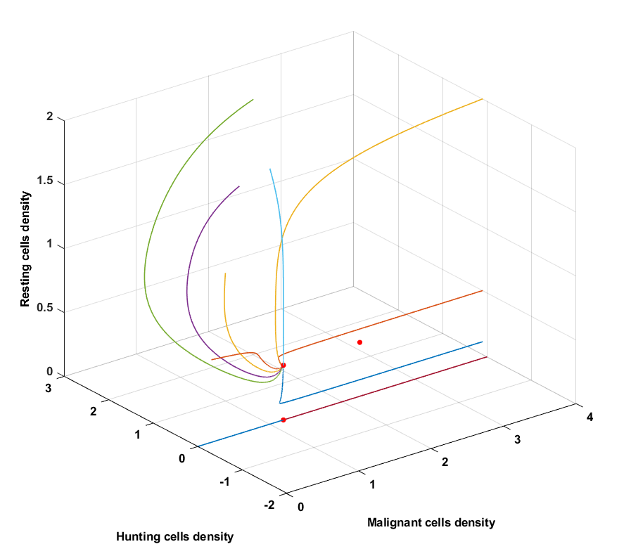
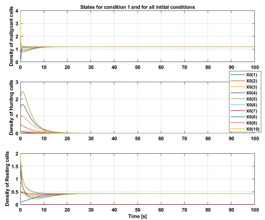
Condition 1 inherent coefficients that are by definition not biologically feasible, because the \(\frac{a_4}{a_3}+\frac{a_7}{a_5} < 1\) inequality does not hold. This implies that condition 1 is not possible and it therefore also causes a fixed point to be excluded from the set $\mathcal{P}$. If the set of conditions were possible, tumor dormancy can be concluded, because a steady state is reached where the malignant, hunting and resting cells remain constant and where the malignant cells are $>0.1$.
Condition 2
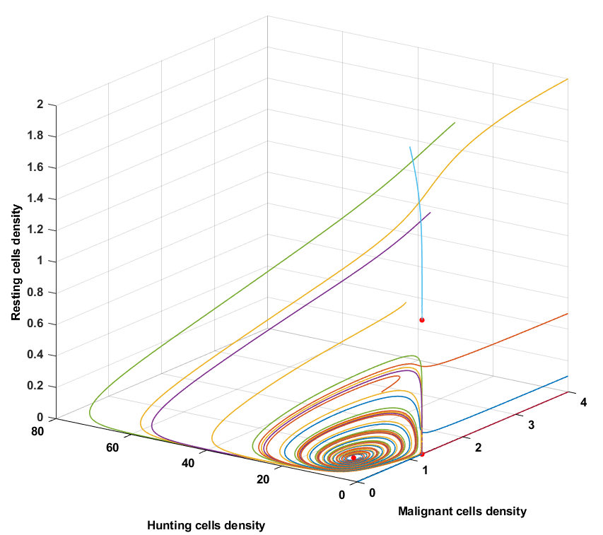
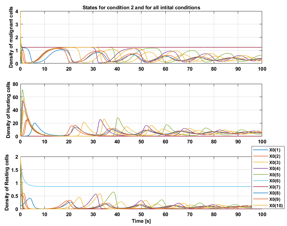
The time trajectories of initial condition \(x_0(1)\) and \(x_0(7)\) converge towards fixed point \(E^*_1\) and the trajectories of initial conditions \(x_0(6)\) converges towards fixed point \(E^*_2\), these are special cases and for that reason also hand picked, because it shows that once the tuple \((M,H,R)\) starts on the M axis, it stays on the M axis. Similarly, once $(M,H,R)$ starts on the $(M,0,R)$ plane it converges towards fixed point \(E^*_2\). Every other initial condition spirals towards the fixed point \(E^*_3\), which implies tumor remission in a cyclic pattern.
Condition 3
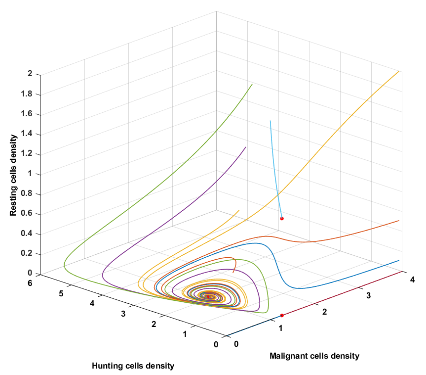
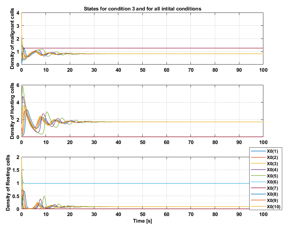
For condition 3 the coefficients $a_5$ and $a_6$ are considerably larger which implies that the growth rate of resting cells have increased as well as the conversion rate from hunting to resting cells. With condition 3, less hunting cells will be available due to the $HR$ term that acts as a balance. The rate of change of hunting cells will therefore overall be smaller that means that the density of hunting cells will overall reach smaller values compared to condition 2. The time of convergence is approximately 6 times faster than condition 2, but the malignant cells reach steady state at a higher value. For condition 3, tumor remission with a cyclic pattern can be concluded.
Stability and contractive properties
For stability analysis, the dynamical system will be linearised. Therefore the Jacobian matrix must be computed:
\[(M, H, R)=(x_1, x_2, x_3)\] \[\dot{x_1}=f_1\left(x_1, x_2, x_3\right) \\ \dot{x_2}=f_2\left(x_1, x_2, x_3\right)\\ \dot{x_3}=f_3\left(x_1, x_1, x_3\right)\] \[\left. A= \begin{bmatrix} \frac{\partial f_1}{\partial x_1} & \frac{\partial f_1}{\partial x_2} & \frac{\partial f_1}{\partial x_3} \\ \frac{\partial f_2}{\partial x_1} & \frac{\partial f_2}{\partial x_2} & \frac{\partial f_2}{\partial x_3} \\ \frac{\partial f_3}{\partial x_1} & \frac{\partial f_3}{\partial x_2} & \frac{\partial f_3}{\partial x_3} \end{bmatrix} \right\vert_{(x_1^{*},x_2^{*},x_3^{*})}\] \[A= \begin{bmatrix} a_1-2a_1M-a_2H & -a2M & 0 \\ 0 & a3R-a_4 & a_3H \\ 0 & -a_6R & a_5-2a_5R-a_6H-a_7 \\ \end{bmatrix}\]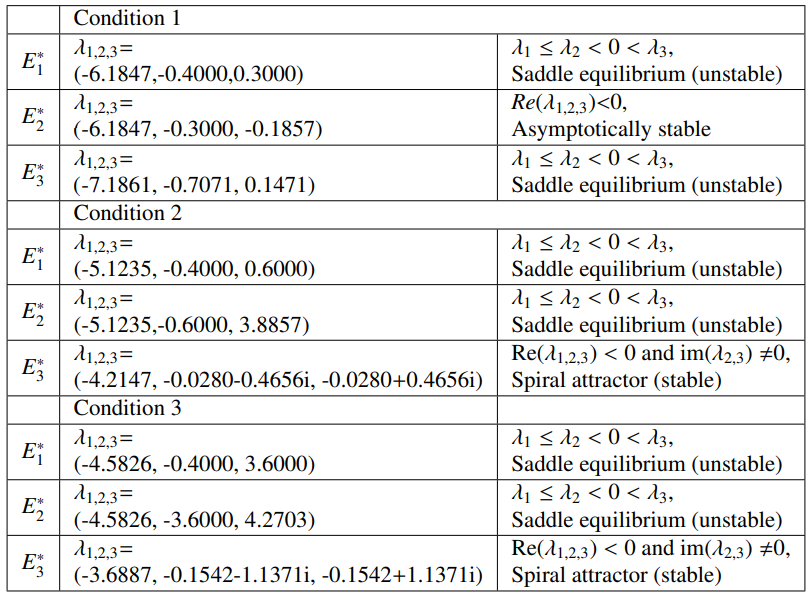
Lyapunov stability
The goal is to find a suitable matrix \(P=P^{\top}\) such that the quadratic function
\[V(M(t), H(t), R(t))=\left(\begin{array}{c} M(t)-M_3^* \\ H(t)-H_3^* \\ R(t)-R_3^* \end{array}\right)^{\top} P\left(\begin{array}{c} M(t)-M_3^* \\ H(t)-H_3^* \\ R(t)-R_3^* \end{array}\right)\]serves as a Lyapanov function to prove stability of the fixed point \(E^*_3\) under condition 3.The suitable value of P can now be solved using convex optimization techniques. For this reason, a mathematical optimization toolbox in Matlab called Yalmip is used to solve semidefinite programming problems using Mosek as a mathematical solver. To following constraints are considered:
- $P=P^{\top}\succ 0$
- $A^{\top} P + P A \prec 0$
Implementing these constraints gave the following result:
\[P=\begin{bmatrix} 0.0855 & 0.0150 & 0.0016\\ 0.0150 & 0.0214 & 0.0170\\ 0.0016 & 0.0170 & 0.8931 \end{bmatrix}\]The Lyapanov function for this specific $P$ holds since $V(x^*)=0$ and $V(x)’<0$. Now that the Lyapanov function is computed, the maximum $\gamma$ in set $\mathcal{V_\gamma}$ can be determined.
\[\mathcal{V}_\gamma:=\left\{(M, H, R) \in \mathbb{R}^3 \mid V(M, H, R) \leq \gamma\right\}\]The maximum level set $\gamma$ can be found via optimization. Here the objective is to maximize $\gamma$ using the following constraints:
- $\left(\begin{array}{c}
M(t)-M_3^*
H(t)-H_3^*
R(t)-R_3^* \end{array}\right)^{\top} P\left(\begin{array}{c} M(t)-M_3^*
H(t)-H_3^*
R(t)-R_3^* \end{array}\right) \leq \gamma$ - $M(t),H(t),R(t) > 0$
- $\gamma>0$
Level sets of the 4-D Lyapunov function can be interpreted as spheres where the maximum $\gamma$ will barely touch the boundaries of set $\mathcal{P}$, since initial conditions outside of the set $\mathcal{P}$ or on the $M,R$ plane won’t converge to $E_3$. The maximum value for the level set of $V(M(t),H(t),R(t))$ and for whom all initial trajectories on this level set still converge is $\gamma_{max}=3.42$.
Time delayed system
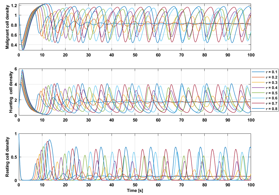
The locations of the fixed points themselves do not change due to the time delay, because these fixed points are solely dependent on the ratio between coefficients $(a_1, … ,a_7)$ and assume all time dependant behavior have died out i.e. the system is not moving $(\dot{M},\dot{H},\dot{R}) = (0,0,0)$. However, the behavior around these fixed points do change with respect to the time delay.
One bifurcation appears between $\tau = 0.2$ and $\tau = 0.3$ for which the fixed point is not an attractive fixed point since the trajectory turns into a limit cycle which orbits around a specific circumference. The higher the time delay the larger this circumference. This bifurcation can be classified by the Hopf bifurcation.

Conclusion & Discussion
Conclusion
Considerable insight into the dynamic behavior of the immune system has been obtained. Depending on the clinical conditions $a_1,…a_7$ biological feasibility can be ensured. For all conditions, the biologically feasible fixed points where asymptotically stable. The only case where asymptotic stability was not ensured is for the time delayed system. In that case, the response is always delayed which results in a limit cycle. The behavior change from asymptotic stability into a limit cycle can be classified as a Hopf bifurcation.
Discussion
Stabilization of the system is not necessary, because the system itself is already asymptotically stable. However, if the dynamics change over time the complete system can be stabilized by linearising around an operating point. Converting the dynamic model into state-space format and check whether the state space is stabilizable. Define a control law $\omega = -K\xi$ for which $A-BK$ is Hurwitz to obtain asymptotic stability.
Software
Main code
%% 5CSA0 Tumor growth assignment
clc, clear all, close all

%% Fixed points
syms M H R a1 a2 a3 a4 a5 a6 a7

f1 = 1+a1*M*(1-M)-a2*M*H == 0;
f2 = a3*H*R-a4*H == 0;
f3 = a5 * R * (1-R) -a6*H*R-a7*R == 0;
solved = solve([f1,f2,f3],[M,H,R]);
% Solve system of equations to find fixed points
for i = 1:length(solved.H)
xstar = [solved.M(i),solved.H(i),solved.R(i)];
xstar_mat{i,1} = xstar;
end
% Reorder to be the same as in the report
xstar_mat([1 2],:) = xstar_mat([2 1],:);
xstar_mat([3 5],:) = xstar_mat([5 3],:);

%% Check biological feasibility
% For all conditions, positive valued states must be achieved at the fixed points
cd1 = [4.5 1 0.5 0.4 0.7 0.2 0.4];
cd2 = [3.5 1 5.0 0.4 0.7 0.1 0.1];
cd3 = [3.0 1 4.8 0.4 3.7 1.9 0.1];
cd = [cd1;cd2;cd3];
coef = [a1 a2 a3 a4 a5 a6 a7];

% Check biological feasibility of the conditions
f4 = (a4/a3) + (a7/a5); % Constraint to be biologically feasible
for k = 1:length(cd(:,1))
    if subs(f4,coef,cd(k,:)) < 1
    feasiblity(k) = 1;
    else
    feasiblity(k) = 0;
    end
end

% Check all fixed point values with conditions
for k = 1:length(cd(:,1))
    for i = 1:length(xstar_mat)
    sol_xstar = double(subs(xstar_mat{i},coef,cd(k,:)));
    sol_xstar_mat{i,k} = sol_xstar;
    end
end

% Remove negative fixed points
sol_xstar_mat_reduced = sol_xstar_mat([1 3 5],:);

% Stability check of the biological feasible fixed points
syms f1_lin f2_lin f3_lin
f1_lin = 1+a1*M*(1-M)-a2*M*H;
f2_lin = a3*H*R-a4*H;
f3_lin = a5 * R * (1-R) -a6*H*R-a7*R;
A = jacobian([f1_lin,f2_lin,f3_lin],[M,H,R]);

% Loop over the coditions (k) and loop over the biologically feasible fixed
% points (i)
for k = 1:length(cd(:,1))
    for i = 1:length(sol_xstar_mat_reduced(1,:))
    A_stab{i,k} = eig(subs(A,[M H R],[sol_xstar_mat_reduced{i,k}]));
    A_stab_numeric{i,k} = double(eig(subs(A,[M,H,R,coef],[sol_xstar_mat_reduced{i,k},cd(k,:)])));
    end
end
% All the eigen values per fixed point per condition in (i_(3x1),k) format
A_eig = cell2mat(A_stab_numeric);
A_num_cd3 = double(subs(A,[M H R coef],[sol_xstar_mat_reduced{3,3} cd(3,:)]));

%% Simulation
t = 0:0.01:100;
% Define initial conditions with first a linear spacing and then some
% arbitrary points of interest
x0_1 = [(0:0.5:2)';1;4;4  ;4;4]';
x0_2 = [(0:0.5:2)';0;0;0.1;0.1;0.1]';
x0_3 = [(0:0.5:2)';2;0;0.1;0.5;2]';
scale_factor = 0.02;
x0 = [x0_1;x0_2;x0_3];
[x1,x2,x3] = meshgrid(0:0.25:2);

%%% Phase plot %%%

for k = 1:length(cd(:,1))
    for p = 1:length(x0)
        x = cell_interaction(t,x0(:,p),cd(k,:));
        solx{p,k} = [x(:,1) x(:,2) x(:,3)];
    end
    % 3D phase plot
    x1dot = 1+cd(k,1).*x1.*(1-x1)-cd(k,2).*x1.*x2;
    x2dot= (cd(k,3).*x2.*x3)-cd(k,4).*x2;
    x3dot= cd(k,5).*x3.*(1-x3)-(cd(k,6).*x2.*x3)-(cd(k,7).*x3);
    figure()
    quiver3(x1,x2,x3,x1dot*scale_factor,x2dot*scale_factor,x3dot*scale_factor,'autoscale','off')
    grid on; axis image;
    xlabel('Malignant cells density')
    ylabel('Hunting cells density')
    zlabel('Resting cells density')
end

%%% Time plot %%%

for k = 1:length(cd(:,1))
figure()
subplot(311)
    for i = 1:length(solx(:,1))
    plot(t,solx{i,k}(:,1))
    hold on; grid on
    end
    str = sprintf("States for condition %d and for all intital conditions",k);
    title(str)
    ylabel('Density of malignant cells')
    subplot(312)

    for i = 1:length(solx(:,1))
    plot(t,solx{i,k}(:,2))
    hold on; grid on
    end

    ylabel('Density of Hunting cells')
    subplot(313)

    for i = 1:length(solx(:,1))
    plot(t,solx{i,k}(:,3))
    hold on; grid on
    legends{i} = sprintf('X0(%d)', i);
    end

    xlabel('Time [s]')
    legend(legends)
    ylabel('Density of Resting cells')
    plotTweak();
end

%%% 3D trajetory plot %%%

for k = 1:length(cd(:,1))
    figure()
    for i = 1:length(solx(:,1))
    plot3(solx{i,k}(:,1),solx{i,k}(:,2),solx{i,k}(:,3))
    hold on
    end
    plot3(sol_xstar_mat{1,k}(1),sol_xstar_mat{1,k}(2),sol_xstar_mat{1,k}(3),'r.', 'MarkerSize', 15)
    plot3(sol_xstar_mat{3,k}(1),sol_xstar_mat{3,k}(2),sol_xstar_mat{3,k}(3),'r.', 'MarkerSize', 15)
    plot3(sol_xstar_mat{5,k}(1),sol_xstar_mat{5,k}(2),sol_xstar_mat{5,k}(3),'r.', 'MarkerSize', 15)
    grid on
    xlabel('Malignant cells density')
    ylabel('Hunting cells density')
    zlabel('Resting cells density')
    plotTweak();
end


%% Time delayed system Q8
t = (0:0.01:100);
% delay_bif = 0.84932; % Include to see crash bifurcation
delay_span = (0.1:0.1:0.8)';
delay_span = [delay_span]; %[delay_span;delay_bif];
delay = [delay_span delay_span delay_span];
% delay = [0.01 0.01 0.01]'
x0 = [1 1 1]';
% delay = [0.1 0.1 0.1];
for i = 1:length(delay(:,1))
sol = d_cell_interaction(t,delay(i,:),x0,cd(3,:));
sol_data{i} = [sol.x;sol.y];
end

figure; clear legends
for k = 1:length(delay(:,1))
plot3(sol_data{k}(2,:),sol_data{k}(3,:),sol_data{k}(4,:))
xlabel('Malignant cells density')
ylabel('Hunting cells density')
zlabel('Resting cells density')
hold on
end
plot3(sol_xstar_mat{1,3}(1),sol_xstar_mat{1,3}(2),sol_xstar_mat{1,3}(3),'r.', 'MarkerSize', 15)
plot3(sol_xstar_mat{3,3}(1),sol_xstar_mat{3,3}(2),sol_xstar_mat{3,3}(3),'r.', 'MarkerSize', 15)
plot3(sol_xstar_mat{5,3}(1),sol_xstar_mat{5,3}(2),sol_xstar_mat{5,3}(3),'r.', 'MarkerSize', 15)
legend('\tau = 0.1','\tau = 0.2','\tau = 0.3','\tau = 0.4','\tau = 0.5','\tau = 0.6','\tau = 0.7','\tau = 0.8','\tau bif.')
grid on

figure;
for i = 1:length(delay(:,1))
plot(sol_data{i}(1,:),[sol_data{i}([2 4],:)])
title('Time response of \tau = 0.1.');
xlabel('time t');
ylabel('solution y');
legend('M','H','R')
hold on
end

figure;
for i = 1:length(delay(:,1))
subplot(311)
plot(sol_data{i}(1,:),sol_data{i}(2,:))
% title('Time responses of (M,H,R) for different \tau');
ylabel('Malignant cell density');
hold on
grid on
subplot(312)
plot(sol_data{i}(1,:),sol_data{i}(3,:))
ylabel('Hunting  cell density');
grid on
hold on
subplot(313)
plot(sol_data{i}(1,:),sol_data{i}(4,:))
ylabel('Resting cell density');
grid on
hold on
xlabel('Time [s]');
end
legend('\tau = 0.1','\tau = 0.2','\tau = 0.3','\tau = 0.4','\tau = 0.5','\tau = 0.6','\tau = 0.7','\tau = 0.8')

%% Lyapunov function
syms x1 x2 x3 p11 p12 p13 p22 p23 p33
Q = eye(3);
x1_star = 0.8260;
x2_star = 1.7325;
x3_star = 0.0833;
xi = [x1-x1_star;x2-x2_star;x3-x3_star];
x = [x1;x2;x3];
P = [p11 p12 p13;
     p12 p22 p23
     p13 p23 p33];

f = transpose(A_num_cd3)*P+P*A_num_cd3;
solveforP = f+Q == 0;
solved_p = solve(solveforP, [p11 p12 p13 p22 p23 p33]);

P = double([solved_p.p11 solved_p.p12 solved_p.p13;
     solved_p.p12 solved_p.p22 solved_p.p23;
     solved_p.p13 solved_p.p23 solved_p.p33]);
V = transpose(xi)*P*(xi);

%% Stabilizing controller
% Find fixed point including u_star
syms M_star H_star R_star a1 a2 a3 a4 a5 a6 a7 u_star
M_star_num = 0.1;
c = subs(coef,coef,cd3);
f1 = 1+c(1)*M_star_num*(1-M_star_num)-c(2)*M_star_num*H_star == 0;
f2 = c(3)*H_star*R_star-c(4)*H_star == 0;
f3 = c(5)*R_star*(1-R_star)-c(6)*H_star*R_star-c(7)*R_star+u_star == 0;

[H_star_num,u_star_num,R_star_num] = solve([f1,f2,f3],[H_star,u_star,R_star]);
fixed_stab = double([M_star_num,H_star_num,R_star_num,u_star_num]);

% Linearize
f1_lin = 1+c(1)*M_star*(1-M_star)-c(2)*M_star*H_star;
f2_lin = c(3)*H_star*R_star-c(4)*H_star;
f3_lin = c(5)*R_star*(1-R_star)-c(6)*H_star*R_star-(c(7)*R_star)+u_star;

A = jacobian([f1_lin,f2_lin,f3_lin],[M_star,H_star,R_star]);
B = jacobian([f1_lin,f2_lin,f3_lin],u_star);

A_num = double(subs(A,[M_star H_star R_star u_star],fixed_stab));
B_num = double(B);

% Check controllability
Contr_mat = ctrb(A_num,B_num);

% Design K such that A-BK is Hurwitz
% pole_loc = [-20 -21 -22];
% pole_loc = [-1 -2 -10];
pole_loc = [-1 -10 -0.1];
K = place(A_num,B_num,pole_loc);
hurwitz = eig(A_num-B_num*K);
F = -K;
% Check whether the controlled system stays in positive invariant set P
states_star = fixed_stab(1:end-1);
input_star = fixed_stab(end);

syms k1 k2 k3 M H R
k = [k1 k2 k3];
f1 = -k * [M-fixed_stab(1);-fixed_stab(2);-fixed_stab(3)]+fixed_stab(4) > 0;
f2 = -k * [-fixed_stab(1);H-fixed_stab(2);-fixed_stab(3)]+fixed_stab(4) > 0;
f3 = -k * [-fixed_stab(1);-fixed_stab(2);R-fixed_stab(3)]+fixed_stab(4) > 0;

%% Simulation controlled system
t = 0:0.001:100;
% Define initial conditions with first a linear spacing and then some
% arbitrary points of interest
xi0_1= (-0.05:0.025:0.05); % Perturbation of Malignant cells
xi0_2 = (-0.05:0.025:0.05); % Perturbation of Hunting cells
xi0_3 = (-0.05:0.025:0.05); % Perturbation of Resting cells

xi0 = [xi0_1;xi0_2;xi0_3];

%%% solver %%%

for p = 1:length(xi0)
    x = stab_cell_interaction(t,xi0(:,p),A_num,B_num,K);
    solx_stab{p} = [x(:,1) x(:,2) x(:,3) ];
end

%%% 3D trajetory plot %%%

figure()
for i = 1:length(solx_stab)
plot3(solx_stab{i}(:,1),solx_stab{i}(:,2),solx_stab{i}(:,3))
hold on
end
grid on
xlabel('Malignant cells density perturbation')
ylabel('Hunting cells density perturbation')
zlabel('Resting cells density perturbation')
plotTweak();

%% From perturbation to actual state simulation plot 3D

figure()
for i = 1:length(solx_stab)
plot3(solx_stab{i}(:,1)+M_star_num,solx_stab{i}(:,2)+double(H_star_num),solx_stab{i}(:,3)+double(R_star_num))
hold on
end
plot3(fixed_stab(1),fixed_stab(2),fixed_stab(3),'r.', 'MarkerSize', 15)
grid on
xlabel('Malignant cells density')
ylabel('Hunting cells density')
zlabel('Resting cells density')
legend('\xi = -0.05','\xi=-0.025','\xi=0','\xi=0.025','\xi=0.05')
plotTweak();

F = -K;

% Plot input
figure()
for i = 1:length(solx_stab)
u_traj =  fixed_stab(4) - K(1)*[solx_stab{i}(:,1)]-K(2)*[solx_stab{i}(:,2)]- K(3)*[solx_stab{i}(:,3)];
plot(t,u_traj)
hold on
grid on
end
xlabel('Time [s]')
ylabel('Control input u(t)')
legend('\xi = -0.05','\xi=-0.025','\xi=0','\xi=0.025','\xi=0.05')
plotTweak();

%% Commands
% set(fig,'renderer','Painters')
% saveas(fig,'figName','epsc')
Functions
cell_interaction.m
function x = cell_interaction(t,x0,cd)
[t,x] = ode45(@coupledfun,t,x0,[],cd);
end
coupledfun.m
function dxdt = coupledfun(t,x0,cd)
x1 = x0(1);
x2 = x0(2);
x3 = x0(3);
dx1dt = 1+cd(1)*x1*(1-x1)-cd(2)*x1*x2;
dx2dt = cd(3)*x2*x3-cd(4)*x2;
dx3dt = cd(5)*x3*(1-x3)-cd(6)*x2*x3-cd(7)*x3;
dxdt = [dx1dt;dx2dt;dx3dt];
end
d_cell_interaction.m
function y = d_cell_interaction(t,delay,x0,cd)
%D_CELL_INTERACTION Summary of this function goes here
%   Detailed explanation goes here
y = dde23(@d_coupledfun,delay,x0,[t(1), t(end)],[],cd);
end
d_history.m
function s = d_history(t,x0)
% Constant history function for DDEX1.
s = x0;
end
d_coupledfun.m
function dydt = d_coupledfun(t,y,Z,cd)
% Differential equations function for DDEX1.
x_lagM = Z(1);
x_lagH = Z(2);
x_lagR = Z(3);
x1 = y(1);
x2 = y(2);
x3 = y(3);
dx1dt = 1+cd(1)*x1*(1-x1)-cd(2)*x1*x2;
dx2dt = cd(3)*x_lagH*x_lagR-cd(4)*x2;
dx3dt = cd(5)*x3*(1-x3)-cd(6)*x2*x3-cd(7)*x3;
dydt = [dx1dt;dx2dt;dx3dt];
stab_cell_interaction.m
function x = stab_cell_interaction(t,x0,A_num,B_num,K)
[t,x] = ode45(@stab_coupledfun,t,x0,[],A_num,B_num,K);
end
stab_coupledfun.m
function dxdt = stab_coupledfun(t,x0,A_num,B_num,K)
x1 = x0(1);
x2 = x0(2);
x3 = x0(3);
dx1dt = A_num(1,:)*[x1;x2;x3] + B_num(1)*(-K*[x1;x2;x3]);
dx2dt = A_num(2,:)*[x1;x2;x3] + B_num(2)*(-K*[x1;x2;x3]);
dx3dt = A_num(3,:)*[x1;x2;x3] + B_num(3)*(-K*[x1;x2;x3]);
dxdt = [dx1dt;dx2dt;dx3dt];
end
Resources
Books
[1.] Khalil, H.K. (2014) Nonlinear systems. Upper Saddle River, NJ: Prentice Hall.