This project focusses on describing the temperature distribution evolution of a 2D plate with as few equations as possible. In particular we will be interested in the heat diffusion process that takes place as a result of individual heat loads $u_1$ and $u_2$ applied on the surface. The equations will be approximated by using a Galerkin projection onto the heat diffusion equation. The fourier basis will be exploited to utilize its orthogonality properties. After which the POD basis will be defined from a high dimensional data set to represent the heat diffusion equations in only a few ordinary differential equations. Before we start with the derivations, in the video below you can see the main results.

Heat diffusion equation

Firstly, the given heat diffusion equation is stated as follows. \(\rho(x, y) c(x, y) \frac{\partial T}{\partial t}(x, y, t)=\left[\begin{array}{ll} \frac{\partial}{\partial x} & \frac{\partial}{\partial y} \end{array}\right] K(x, y)\left[\begin{array}{l} \frac{\partial T(x, y, t)}{\partial x} \\ \frac{\partial T(x, y , t)}{\partial y} \end{array}\right]+u(x, y, t)\) Where,

• $T(x,y,t)$ ~ $[K]$ is the temperature in Kelvin.
• $\rho(x,y)$ ~ $[kg/m^3]$ is the density of the plate.
• $c(x,y)$ ~ $[J/(kg K)]$ is the heat capacity.
• $K(x,y)$ ~ $[W/(mK)]$ is the location dependent thermal conductivity matrix, which is positive definite.
• $u(x,y,t)$ ~ $[W/m^2]$ is the input heat flux into the plate.

For the rest of the project the plate is assumed to be isotropic and homogeneous.

Fourier basis

The inner product will be defined as follows:

\[\left\langle \varphi_i,\varphi_j \right\rangle:=\int_0^{L_x}\int_0^{L_y}\varphi_i(x,y)\varphi_j(x,y)dydx.\]

$\varphi_{k,l}$ represents the product of $\varphi_k(x)$ and $\varphi_l(y)$, which are defined as follows for non-negative integers $k$ and $l$

\[\varphi_k(x) = \begin{cases} \;\frac{1}{\sqrt{L_x}}\;\;\;\;\;\;\;\;\;\;\;\;\;\;\;\;\;\;\;\;\;\text{if}\;k=0\\ \sqrt{\frac{2}{L_x}}\cos\left(\frac{k\pi x}{L_x}\right)\;\;\;\;\;\text{if}\;k>0 \end{cases} \;\;\;\;\;\;\;\;\;\; \varphi_l(y) = \begin{cases} \;\frac{1}{\sqrt{L_y}}\;\;\;\;\;\;\;\;\;\;\;\;\;\;\;\;\;\;\;\;\text{if}\;l=0\\ \sqrt{\frac{2}{L_y}}\cos\left(\frac{l\pi y}{L_y}\right)\;\;\;\;\;\text{if}\;l>0 \end{cases}\]

Galerkin projection

We use the Galerkin projection to derive, for arbitrary $k$ and $l$, an explicit ordinary differential equation for the coefficient function $a_{k,l}(t)$ in the spectral expansion given as:

\[T(x,y,t)=\sum_{k=0}^\infty\sum_{l=0}^\infty a_{k,l}(t)\varphi_{k,l}(x,y)\]

The Galerkin projection of the homogeneous model is taken as follows

\[\left\langle \rho c \frac{\partial}{\partial t}T(x,y,t),\varphi_{k,l} \right\rangle= \left\langle \kappa \left(\frac{\partial^2}{\partial x^2}T(x,y,t)+\frac{\partial^2}{\partial y^2}T(x,y,t)\right) + u(x,y,t),\varphi_{k,l} \right\rangle\]

Now, the spectral expansion is substituted into the Galerkin projection. However, the non-negative integers $k$ and $l$ of this spectral expansion are changed to $p$ and $q$ respectively, since $k$ and $l$ in are different. Doing this results in

\[\begin{aligned} &\left\langle \rho c \frac{\partial}{\partial t}\sum_{p=0}^\infty\sum_{q=0}^\infty a_{p,q}(t)\varphi_{p,q}(x,y),\varphi_{k,l}(x,y) \right\rangle=\\ &\left\langle \kappa \left(\frac{\partial^2}{\partial x^2}\sum_{p=0}^\infty\sum_{q=0}^\infty a_{p,q}(t)\varphi_{p,q}(x,y)+\frac{\partial^2}{\partial y^2}\sum_{p=0}^\infty\sum_{q=0}^\infty a_{p,q}(t)\varphi_{p,q}(x,y)\right) + u(x,y,t),\varphi_{k,l}(x,y) \right\rangle \end{aligned}\]

Due to linearity of the inner product, the summations can be taken out of the inner product, moreover the $x$, $y$ and $t$ dependencies are dropped for ease of notation, this gives

\[\rho c \frac{\partial}{\partial t}\sum_{p=0}^\infty\sum_{q=0}^\infty a_{p,q}\left\langle \varphi_{p,q},\varphi_{k,l} \right\rangle= \kappa\sum_{p=0}^\infty\sum_{q=0}^\infty a_{p,q}\left\langle \frac{\partial^2}{\partial x^2}\varphi_{p,q}+\frac{\partial^2}{\partial y^2}\varphi_{p,q},\varphi_{k,l}\right\rangle + \left\langle u,\varphi_{k,l} \right\rangle\]

Since $\varphi_{p,q}$ is a product of the two basis functions, the two double partial derivatives with respect to $x$ and $y$ position can be rewritten to $\ddot\varphi_p\varphi_q + \varphi_p \ddot\varphi_q$. Additionally, the partial derivative with respect to time of $a_{p,q}$ is rewritten as $\dot a_{p,q}$. The expression therefore becomes:

\[\rho c \sum_{p=0}^\infty\sum_{q=0}^\infty \dot a_{p,q} \left\langle \varphi_{p,q},\varphi_{k,l} \right\rangle= \kappa\sum_{p=0}^\infty\sum_{q=0}^\infty a_{p,q}\left\langle \ddot\varphi_p\varphi_q + \varphi_p \ddot\varphi_q,\varphi_{k,l}\right\rangle + \left\langle u,\varphi_{k,l} \right\rangle\]

Due to the orthonormality of $\varphi_{k,l}$, the summation on the left-hand side of the equation will only result in non-zero values when $p$ and $q$ are equal to $k$ and $l$ respectively. This gives the following expression for $\dot a_{k,l}$.

\[\dot a_{k,l} =\frac{\kappa}{\rho c}\sum_{p=0}^\infty\sum_{q=0}^\infty a_{p,q}\left\langle \ddot\varphi_p\varphi_q + \varphi_p \ddot\varphi_q,\varphi_{k,l}\right\rangle + \frac{1}{\rho c}\left\langle u,\varphi_{k,l} \right\rangle\]

Next up, evaluation of $\ddot\varphi_p\varphi_q + \varphi_p \ddot\varphi_q$ for different values of $p$ and $q$. This is done through fourier basis functions, keep in mind that $\ddot\varphi_p$ is the second partial derivative with respect to $x$ position and $\ddot\varphi_q$ is the second partial derivative with respect to $y$ position.

\[\begin{aligned} &\ddot\varphi_p\varphi_q + \varphi_p \ddot\varphi_q = 0\;\;\;\;\;\;\;\;\;\;\;\;\;\;\;\;\;\;\;\;\;\;\;\;\;\;\;\;\;\;\;\;\;\;\;\;\;\;\; \text{if}\;\;p = 0\;\;\text{and}\;\;q = 0\\ &\ddot\varphi_p\varphi_q + \varphi_p \ddot\varphi_q = -\frac{p^2\pi^2}{L_x^2}\varphi_{p,q}\;\;\;\;\;\;\;\;\;\;\;\;\;\;\;\;\;\;\;\;\;\;\;\;\; \text{if}\;\;p > 0\;\;\text{and}\;\;q = 0\\ &\ddot\varphi_p\varphi_q + \varphi_p \ddot\varphi_q = -\frac{q^2\pi^2}{L_y^2}\varphi_{p,q}\;\;\;\;\;\;\;\;\;\;\;\;\;\;\;\;\;\;\;\;\;\;\;\;\; \text{if}\;\;p = 0\;\;\text{and}\;\;q > 0\\ &\ddot\varphi_p\varphi_q + \varphi_p \ddot\varphi_q = -\left(\frac{p^2\pi^2}{L_x^2}+\frac{q^2\pi^2}{L_y^2}\right)\varphi_{p,q}\;\;\;\;\;\; \text{if}\;\;p > 0\;\;\text{and}\;\;q > 0\\ \end{aligned}\]

By looking at the expressions above, it can be concluded that the fourth expression, describing the case in which both $p$ and $q$ are greater than zero, also holds for the cases when $p$ or $q$ are equal to zero. Thus, all cases converge towards.

\[\dot a_{k,l} =-\frac{\kappa}{\rho c}\left(\frac{p^2\pi^2}{L_x^2}+\frac{q^2\pi^2}{L_y^2}\right)\sum_{p=0}^\infty\sum_{q=0}^\infty a_{p,q}\left\langle \varphi_{p,q},\varphi_{k,l}\right\rangle + \frac{1}{\rho c}\left\langle u,\varphi_{k,l} \right\rangle\]

Through the property of orthonormality of $\varphi_{k,l}$, this expression can again be rewritten

\[\dot a_{k,l}=-\frac{\kappa}{\rho c}\left( \frac{k^2\pi^2}{L_x^2}+\frac{l^2\pi^2}{L_y^2}\right) a_{k,l}+ \frac{1}{\rho c}\left\langle u,\varphi_{k,l} \right\rangle\]

Writing out the standard inner product of $u$ and $\varphi_{k,l}$, and Substituting back in the time and position dependencies gives

\[\dot a_{k,l}(t)=-\frac{\kappa}{\rho c}\left( \frac{k^2\pi^2}{L_x^2}+\frac{l^2\pi^2}{L_y^2}\right) a_{k,l}(t)+ \frac{1}{\rho c}\left\langle u(x,y,t),\varphi_{k,l}(x,y) \right\rangle\]

Therefore, a system of completely decoupled ordinary differential equations is found for the coefficient function $a_{k,l}(t)$.

Simulation

Initial conditions

Three different initial temperature profiles will be experimented with.

• Gaussian distributed temperature profile
• Block profile
• Fourier basis profile

Simulation without input

For animations I would like to refer you to the youtube link on the top of the post.

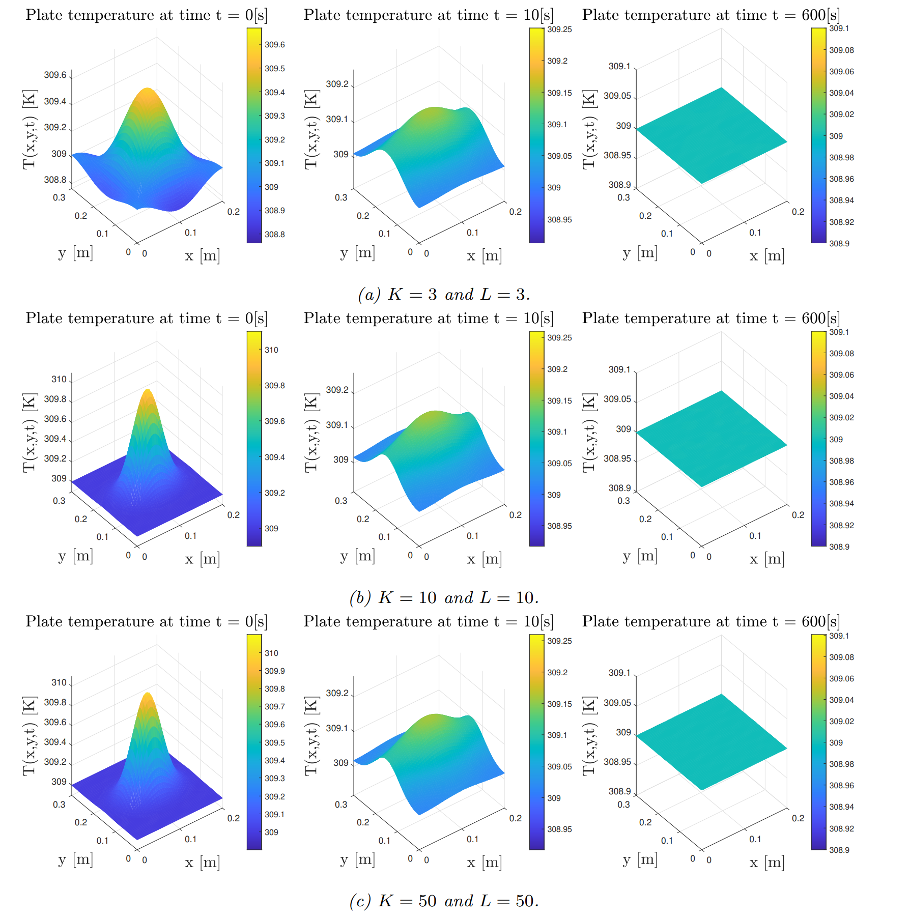
The temperature distributions on the plate, simulated at different points in time, for different values of $K$ and $L$, are given in the figure above. From this figure, it becomes clear that adding additional basis functions, through higher values of $K$ and $L$, has diminishing returns. This is at least the case for the initial temperature profile that was chosen. The figure where both $K$ and $L$ are equal to $3$, shows that approximation of the initial temperature profile is poor due to each direction of the plane being only approximated by a few cosine functions. Creating a disparity between $K$ and $L$ results in one axis being approximated by more distinct basis functions than the other axis.

Simulation with input

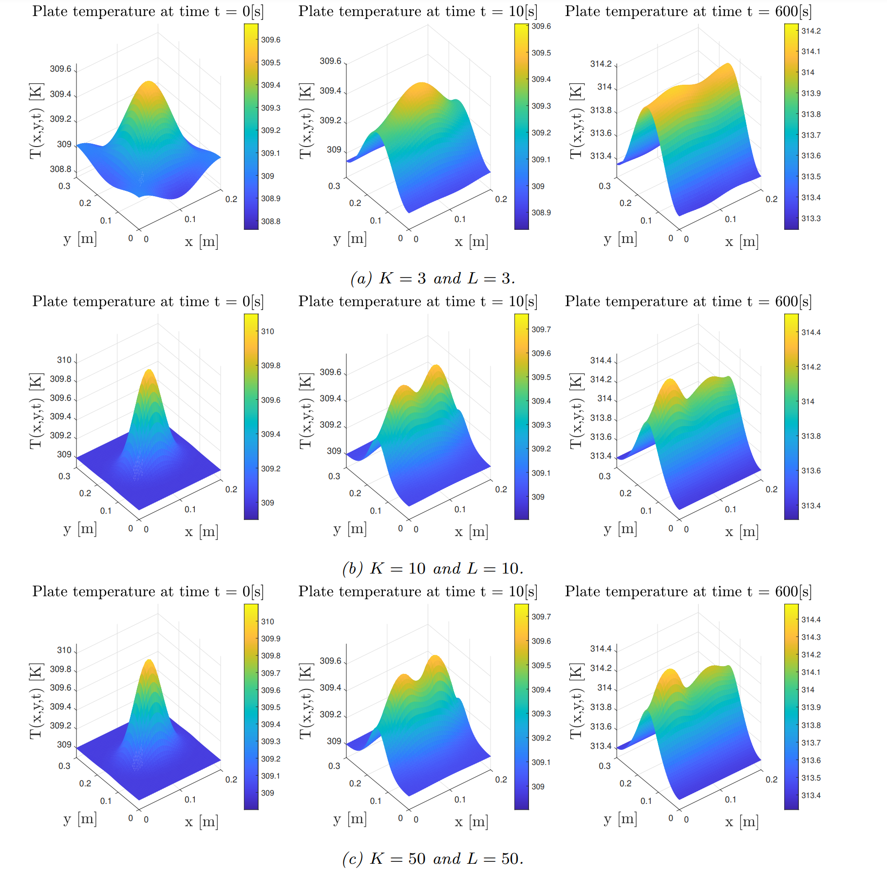The temperature evolution of the same Gaussian initial heat profile from previous section is depicted for varying $K$ and $L$. The input heat sources are given as the absolute values of time-depending sinusoidal functions, with an amplitude of $0.4$ Kelvin. A phase difference of $90^o$ was chosen between $u_1(t)$ and $u_2(t)$. From these figures, it be becomes clear that the lowest order truncation ($K=L=3$) performs poorly, whilst the higher order truncations ($K=L=10$ and $K=L=50$) perform nearly identical. In contrast to previous section, the heated plate can never settle at a homogeneous temperature as long as the input is nonzero. After most of the dynamics of the initial condition have settled, a ridge shaped temperature profile can be seen. This shape is the result of the plate being longer in the $y$-direction, as well as the imposed boundary conditions. Additionally, the continuous input of heat, without any heat loss to the environment, causes the average plate temperature to rise over time.

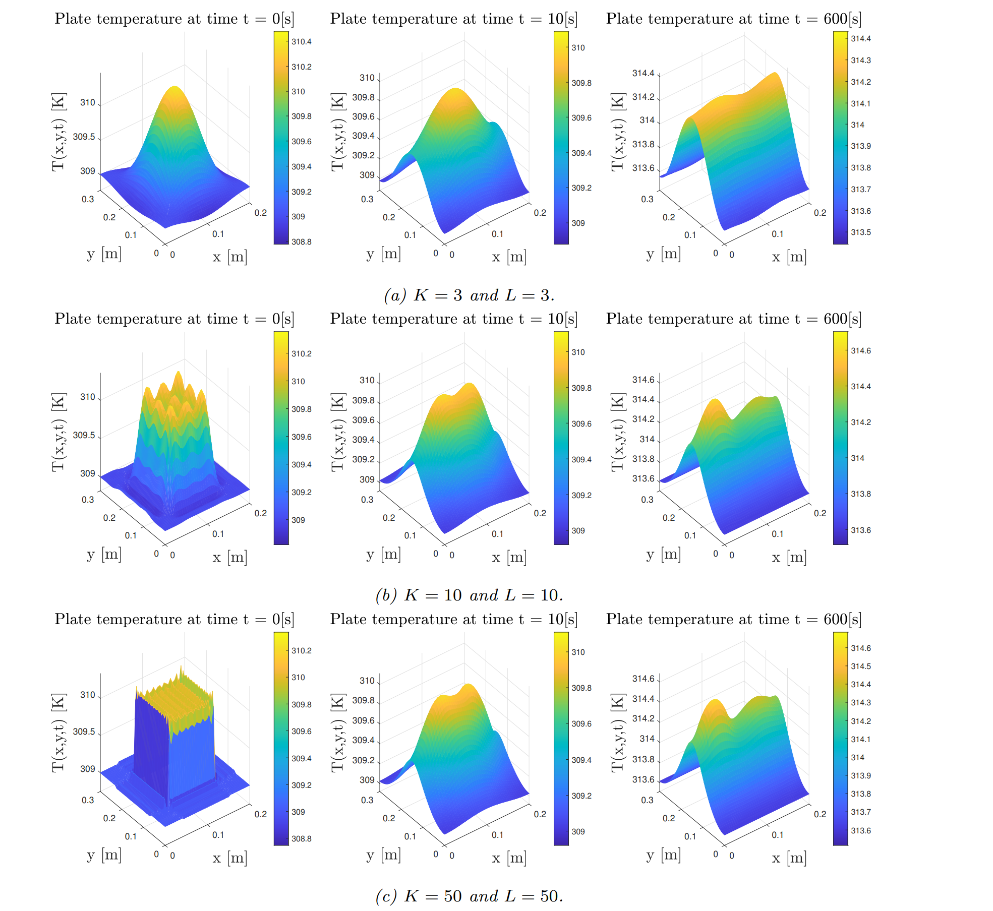The temperature evolution for the heated-plate with an initial block-shaped temperature profile is shown above. In contrast to the Gaussian initial temperature profile, this shape is a lot harder to be approximated through the cosine basis functions. Higher truncation orders have significantly better performance in this case.

The figure above depicts the initial temperature profile that was described through the basis functions. This is not a realistic temperature distribution, and therefore not of much interest. However, it is still interesting to see that the approximation of the initial profile would be very accurate when $K$ and $L$ are greater than, or equal to the order used for the initial temperature profile, and not accurate if $K$ and $L$ would be smaller.

It can be concluded that the shape of the initial temperature profile has a large effect on the accuracy of the truncated model. Truncation of order 3 have very limited performance, whereas truncations of order 10 are able to capture the main dynamics of interest. Order 50 truncations are able to approximate square shapes with reasonably high precision.

POD basis

To even further reduce the number of ordinary differential equations that are required to represent the diffusion behavior, the POD basis will be used. POD stands for proper orthogonal decomposition, which is a technique to reduce the order of complexity by looking at the singular value decomposition of high dimensional data and only focussing on dominant behavior. In this project the fourier basis with $K=50$ and $L=50$ is used to create a matrix of snapshots. Where the rows represent the spatial data and the columns represent temporal data. Since this problem is 2-dimensional the spatial data is stacked. The SVD is defined as follows. \(W_{snap}=U \Sigma V^T\) Where U and V are unitary rotation matrices and sigma is a diagonal matrix that contains the ordered singular values. After using the singular value decomposition and scaling it by the proper discretization constants, the new basis functions in the most dominant directions will reveal inside of the U matrix. These vectors are also ordered in dominance from left to right. Where the most left vector is the most dominant. The first three dominant shapes are shown below. To see the advantage of the POD basis compared to the Fourier basis, I took the block shape as the initial condition. The POD basis can represent block like behavior with $R = 13$ modes compared to $K=50$ and $L=50$ that was required for the fourier basis, because it is not constrained by only sinusoidal functions. Comparison for $R = 5$ and $R = 13$ is shown below.

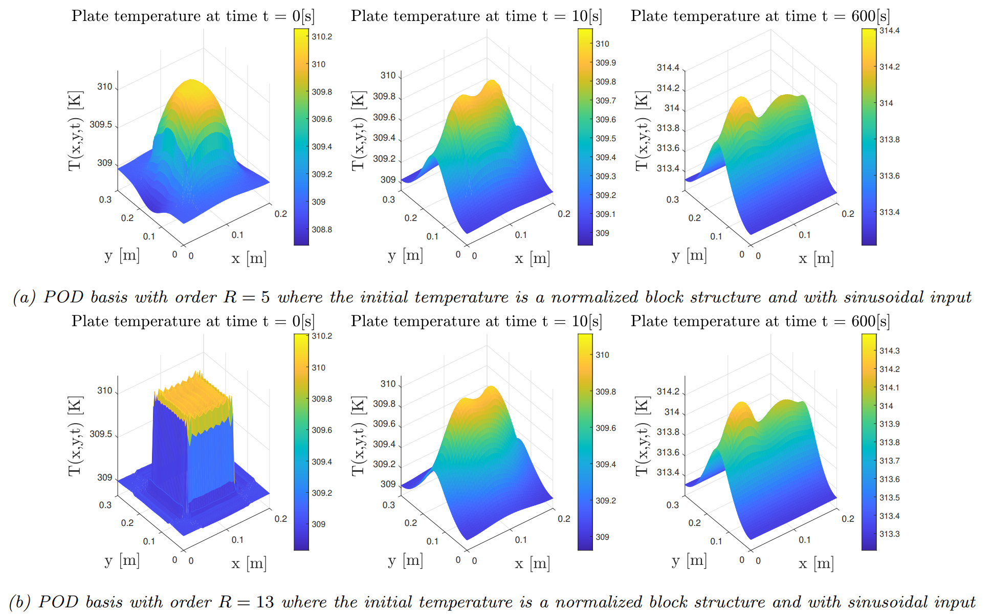
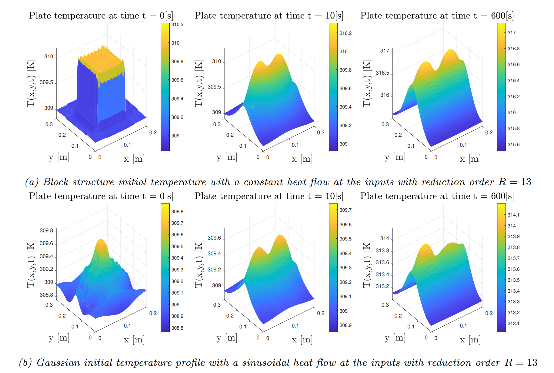
To test the performance of the POD basis compared to the fourier basis when we simulate it with different initial conditions and different input behavior than was shown in the snapshot matrix. This implies that the POD basis must simulate the diffusion behavior with modes that it has not seen before. This is clearly visible in the figure below. In a) the initial condition is the same as in the snapshot matrix, but the input now is constant instead of sinusoidal, which causes the residual compared to b) in the figure above to grow over time. Since the input is different this is to be expected. In the case of b) the input is the same as the snapshot matrix, but the initial condition is forced to be Gaussian. This shows that the POD basis poorly describes the gaussian initial condition, because this mode is not contained in the snapshot matrix. However, after the initial behavior has died out, this scenario resembles the snapshot matrix again since the input is the same.

Conclusion & Recommendations

To conclude, the POD basis can drastically reduce the model order. However, care should be taken with models that vary in time, since the POD basis is only as good as the data that represents the actual spatial-temporal behavior of the true system.

The code can be extended to also work for non-homogeneous heat diffusion. The $\rho(x,y)c(x,y)$ as well as $\kappa(x,y)$ must be continuous and differentiable in $x$ and $y$ in order to model it as a linear PDE.

Resources

Software

If you are interested in the source code from this project, I invite you to take a look at my Repository.

Tutorials

All video lectures of Steve Brunton and Nathan Kutz were very helpful in order to understand the basics of POD and model reduction in general.